


Flight Dynamics & Controls
Stability and control of aircraft and spacecraft: axes and moments, static stability and trim, lateral-directional stability, dynamic modes, transfer functions, time response, feedback and PID control, stability margins, and spacecraft attitude control, with six labs. Free, self-paced, and tied to NASA’s X-59, Hubble and Dragonfly.
Courses › AERO 420
About this course
This is a free self-study course outline written by Saving Planets. It is not a university course, it carries no academic credit, and no school is involved.
Its scope follows a one-semester senior flight dynamics and controls course for aerospace engineers. It is modeled on the topics and depth of MIT 16.333 Aircraft Stability and Control, MIT 16.06 Principles of Automatic Control and MIT 16.30 Feedback Control Systems (free on MIT OpenCourseWare), using NASA Glenn’s free Beginner’s Guide to Aeronautics, which we link where it helps. None of those authors, schools or agencies endorses this page.
What we add: every unit ties to real work with a cited public source (NASA’s X-59 flight tests, Hubble’s pointing system and the Dragonfly rotorcraft), every number on the page is re-computed by a checking script before it goes live, and every lab has a free simulation or a spreadsheet.
Work through it in order. Each unit has goals, key ideas, equations, step-by-step examples, practice with full answers, common mistakes, flashcards and a quiz. Your progress is saved only in this browser.
How this course helps save the planet
Stable, well-controlled vehicles fly efficient paths, and the same control ideas point Earth-observing satellites and telescopes precisely enough to measure our planet and universe.
Control engineering also makes new, quieter and more autonomous aircraft possible. Each unit ends with a short, sourced section. Values that are not from a source are labeled as sample or textbook values.
Before you start
Prerequisites
- Dynamics: rigid-body rotation, moments of inertia and angular momentum.
- Differential Equations: linear ODEs and the Laplace transform.
- Linear Algebra: matrices and eigenvalues.
- Aerodynamics I and Aircraft Performance: lift, drag, moments and turning flight.
How to study
- Draw the body axes and the center of gravity before writing any moment equation.
- Keep angles in radians inside formulas; convert to degrees only for the answer.
- Separate static stability (the first tendency after a disturbance) from dynamic stability (what happens over time).
- Sketch the poles in the s-plane for every system you meet.
- Check every answer against physical sense: stable systems settle, unstable ones grow.
- Do every practice problem on paper before opening the answer, and retake the quizzes a few days later.
Lab equipment (for the wet labs)
- A computer or tablet for the free PhET Balancing Act and Masses and Springs simulations.
- Spreadsheet software (any free one works), or Python.
- NASA Glenn’s Beginner’s Guide to Aeronautics pages in a web browser.
- A calculator.
Suggested 15-week schedule
About 6 to 9 hours a week: reading, practice problems and, in lab weeks, the lab.
| Week | Unit | Topics | Reading |
|---|---|---|---|
| 1 | Axes, Rotations and Moments | Axes, cg and moments; Lab A | NASA Glenn |
| 2 | Longitudinal Static Stability | Longitudinal static stability | MIT 16.333 |
| 3 | Trim and Elevator Control | Trim and elevator; Lab B | NASA Glenn |
| 4 | Lateral-Directional Stability and Turns | Lateral-directional stability and turns | MIT 16.333 |
| 5 | Equations of Motion and Dynamic Modes | Equations of motion and linearization | MIT 16.333 |
| 6 | Equations of Motion and Dynamic Modes | Dynamic modes; Lab C | MIT 16.333 |
| 7 | Laplace Transforms and Transfer Functions | Transfer functions; midterm practice | MIT 16.06 |
| 8 | Second-Order Time Response | Second-order response; Lab D | MIT 16.06 |
| 9 | Feedback and PID Control | Feedback and PID | MIT 16.06 |
| 10 | Feedback and PID Control | Autopilot design; Lab E | MIT 16.30 |
| 11 | Stability Analysis: Routh, Root Locus and Margins | Routh, root locus and margins | MIT 16.06 |
| 12 | Spacecraft Attitude Determination and Control | Attitude dynamics and sensors | MIT 16.30 |
| 13 | Spacecraft Attitude Determination and Control | Reaction wheels and slews; Lab F | NASA Hubble |
| 14 | Spacecraft Attitude Determination and Control | Autonomy and fault response | NASA Dragonfly |
| 15 | Spacecraft Attitude Determination and Control | Review; final practice | MIT 16.06 |
Your progress
Tick units and labs as you finish them, and take the quizzes. Progress and quiz scores are saved only in this browser, never sent to us.
Turn on JavaScript to track progress.
Unit 1 · Week 1
Axes, Rotations and Moments
Body axes through the center of gravity, roll, pitch and yaw, control surfaces and the moments they make, finding the center of gravity, and Euler angles.
Learning objectives
By the end of this unit you can:
- Define the roll, pitch and yaw axes.
- Locate a center of gravity from component masses.
- Compute the moment of a control force.
- Match each control surface to its moment.
Key concepts
- In flight an aircraft rotates about its center of gravity (cg), the average location of its mass.
- Body axes: roll toward the nose, pitch toward the right wing tip, yaw toward the bottom of the aircraft.
- Control surfaces make aerodynamic forces at a distance from the cg, producing moments: elevators pitch, the rudder yaws, ailerons roll.
- The cg of several masses is x_cg = Σm_ix_i/Σm_i; moving it changes stability and control.
- Euler angles (yaw ψ, pitch θ, roll φ, applied in that order) describe attitude relative to the Earth.
Key equations
Worked examples, step by step
Example 1.1 A tail force of 2000 N acts 6 m behind the cg (sample values). Find the pitching moment.
Show the steps
- M = 2000 × 6.
Answer: 12,000 N·m.
Example 1.2 Masses of 1000 kg at 2 m, 500 kg at 6 m and 300 kg at 10 m from the nose (sample values). Find the cg.
Show the steps
- Σm = 1800 kg.
- Σmx = 2000 + 3000 + 3000 = 8000 kg·m.
Answer: x_cg = 4.44 m.
Example 1.3 Which surface rolls the aircraft?
Show the steps
- Ailerons deflect in opposite directions on each wing.
Answer: Ailerons produce a rolling moment.
Practice problems
Work each on paper first, then check.
Moment of 500 N at 4 m?
Show answer
2000 N·m.
Which surface yaws the nose?
Show answer
The rudder.
Add 200 kg at 10 m to the example. New cg?
Show answer
10,000/2000 = 5.0 m.
About which point does a kite rotate?
Show answer
Its bridle point.
Common misconceptions
Myth: Aircraft rotate about their nose.
Actually: They rotate about the cg.
Myth: Elevators roll the aircraft.
Actually: They pitch it.
Myth: Euler angle order does not matter.
Actually: Rotations do not commute.
Flashcards
cg
Average location of mass.
Roll
Rotation about the nose axis.
Pitch
Nose up or down.
Yaw
Nose side to side.
Moment
Force × distance.
Euler angles
ψ, θ, φ.
Self-check quiz
How this helps save the planet
NASA Glenn explains that control surfaces produce forces at their centers of pressure, some distance from the cg, creating torques about the principal axes: elevators pitch, the rudder yaws and ailerons roll. The first aircraft to show active control about all three axes was the Wrights’ 1902 glider.
Every modern efficient airliner and Earth-observing aircraft still uses those three moments, now often commanded through flight-control computers.
On Saving Planets: Aerodynamics I · Dynamics
Sources: NASA Glenn Beginner’s Guide: Aircraft rotations · NASA Glenn Beginner’s Guide: Center of gravity
Free learning resources
- NASA Glenn Beginner’s Guide: Aircraft rotations: Free NASA explainer.
- MIT OpenCourseWare 16.333 Aircraft Stability and Control (Fall 2004): Free MIT lectures.
Unit 2 · Week 2
Longitudinal Static Stability
Pitching-moment coefficient, the stability derivative C_mα, the neutral point, static margin, and how cg position and tail size set stability.
Learning objectives
By the end of this unit you can:
- State the condition for static pitch stability.
- Compute static margin.
- Relate static margin to C_mα.
- Explain the effect of moving the cg.
Key concepts
- Static stability is the first tendency after a disturbance: a statically stable aircraft makes a moment that pushes it back.
- In pitch this needs C_mα < 0: more angle of attack makes a nose-down moment.
- The neutral point is the cg location where C_mα = 0.
- Static margin SM = (x_np − x_cg)/c̄; positive means stable. Approximately C_mα = −C_Lα × SM.
- Moving the cg aft reduces stability and control forces; too far aft makes the aircraft unstable unless a computer stabilizes it.
Key equations
Worked examples, step by step
Example 2.1 The neutral point is at 0.35c̄ and the cg at 0.25c̄ (sample values). Find the static margin.
Show the steps
- SM = 0.35 − 0.25.
Answer: SM = 0.10 (10%).
Example 2.2 With C_Lα = 5.5 per radian, find C_mα.
Show the steps
- C_mα = −5.5 × 0.10.
Answer: C_mα = −0.55 per radian: stable.
Example 2.3 Move the cg to 0.30c̄. Find the new C_mα.
Show the steps
- SM = 0.05; −5.5 × 0.05.
Answer: −0.275 per radian: half as stiff.
Practice problems
Work each on paper first, then check.
SM with cg at 0.35c̄?
Show answer
0: neutrally stable.
Sign of C_mα for cg at 0.40c̄?
Show answer
Positive: unstable.
Does a bigger tail move the neutral point fore or aft?
Show answer
Aft, raising static margin.
Why fly with small margins?
Show answer
Less trim drag and lighter controls.
Common misconceptions
Myth: Static stability guarantees dynamic stability.
Actually: It is only the first tendency.
Myth: Aft cg is always safer.
Actually: It reduces stability.
Myth: C_mα should be positive.
Actually: Negative is stable.
Flashcards
Static stability
First tendency to return.
C_mα
Pitch stiffness.
Neutral point
cg where C_mα = 0.
Static margin
(x_np − x_cg)/c̄.
Mean chord c̄
Reference length.
Relaxed stability
Small or negative margin with computer help.
Self-check quiz
How this helps save the planet
NASA reports that after 25 flights the X-59’s real-world flight characteristics closely match simulations, including its flying qualities and its stability margin, which NASA describes as how close the aircraft is to becoming unstable under certain conditions.
The X-59 is shaped to turn a loud sonic boom into a quiet thump, and confirming its stability margin in flight is part of proving that quieter supersonic flight is practical.
On Saving Planets: Aerodynamics I · Aircraft Performance
Sources: NASA: X-59 aircraft builds momentum through 25th flight (Sept. 4, 2026)
Free learning resources
- MIT OpenCourseWare 16.333 Aircraft Stability and Control (Fall 2004): Free MIT lectures.
- NASA Glenn Beginner’s Guide: Center of gravity: Free NASA explainer.
Unit 3 · Week 3
Trim and Elevator Control
Trim as zero net pitching moment, elevator effectiveness, the elevator angle to trim, tail download and trim drag, and stick-fixed versus stick-free stability.
Learning objectives
By the end of this unit you can:
- Write the trim condition.
- Solve for elevator angle to trim.
- Explain why tails often push down.
- Describe trim drag.
Key concepts
- Trim means zero net pitching moment: C_m = C_m0 + C_mα α + C_mδe δ_e = 0.
- Elevator effectiveness C_mδe is negative for a tail elevator: trailing edge down gives nose down.
- The elevator lift acts some distance from the cg, so it makes a torque and the aircraft rotates about its cg.
- Modern tails often carry negative lift to keep the nose up, which the wing must offset with extra lift.
- That extra lift costs induced drag, called trim drag; a smaller static margin reduces it.
Key equations
Worked examples, step by step
Example 3.1 C_m0 = 0.05, C_mα = −0.55, C_mδe = −1.2 per radian (sample values). Find δ_e to trim at α = 0.05 rad.
Show the steps
- 0.05 − 0.0275 − 1.2δ_e = 0.
- δ_e = 0.0225/1.2.
Answer: δ_e = 0.01875 rad = 1.07°.
Example 3.2 What angle of attack trims with zero elevator?
Show the steps
- α = 0.05/0.55.
Answer: α = 0.0909 rad = 5.21°.
Example 3.3 Find C_L at that trim with C_Lα = 5.5.
Show the steps
- 5.5 × 0.0909.
Answer: C_L = 0.50.
Practice problems
Work each on paper first, then check.
δ_e to trim at α = 0.1 rad?
Show answer
−0.00417 rad (−0.24°).
Sign convention for δ_e?
Show answer
Trailing edge down positive.
Why does tail download cost fuel?
Show answer
The wing makes more lift, adding induced drag.
Where was the Wright Flyer’s elevator?
Show answer
At the front.
Common misconceptions
Myth: Trim means level flight.
Actually: It means zero net moment at any steady condition.
Myth: Tails always lift upward.
Actually: Many push down.
Myth: Elevator only changes pitch angle.
Actually: It sets the trimmed angle of attack and speed.
Flashcards
Trim
Zero net moment.
C_mδe
Elevator effectiveness.
Elevator
Pitch control surface.
Tail download
Negative tail lift.
Trim drag
Drag from trimming.
Canard
Forward elevator surface.
Self-check quiz
How this helps save the planet
NASA Glenn explains that the horizontal stabilizer on modern aircraft is usually set at a negative angle, making a downward force that keeps the tail down and the airplane trimmed, and that this negative force must be overcome with greater lift from the wing.
Every bit of extra lift adds drag and fuel burn, so careful trim and cg management are small but real ways to cut aviation emissions.
On Saving Planets: Aircraft Performance · Solutions
Sources: NASA Glenn Beginner’s Guide: Aircraft elevator interactive
Free learning resources
- NASA Glenn Beginner’s Guide: Aircraft elevator interactive: Free NASA interactive.
- MIT OpenCourseWare 16.333 Aircraft Stability and Control (Fall 2004): Free MIT lectures.
Unit 4 · Week 4
Lateral-Directional Stability and Turns
Weathercock (directional) stability, dihedral effect, aileron roll control, roll damping and the roll mode, adverse yaw, and the coordinated turn.
Learning objectives
By the end of this unit you can:
- State directional and roll stability conditions.
- Compute roll-mode time constant and steady roll rate.
- Find bank angle and load factor for a coordinated turn.
- Explain adverse yaw.
Key concepts
- Directional (weathercock) stability needs C_nβ > 0: a sideslip yaws the nose back into the wind.
- Dihedral effect needs C_lβ < 0: a sideslip rolls the aircraft away from the slip.
- Ailerons deflect oppositely to make a rolling moment; roll damping L_p resists roll rate, giving the roll mode with τ = 1/|L_p|.
- The down-going aileron makes more lift and drag, yawing the nose away from the turn (adverse yaw); the rudder fixes it.
- In a coordinated level turn tan φ = V²/(gR) and load factor n = 1/cos φ.
Key equations
Worked examples, step by step
Example 4.1 A turn at 100 m/s with radius 2000 m (sample values). Find the bank angle.
Show the steps
- tan φ = 100²/(9.80665 × 2000) = 0.510.
Answer: φ = 27.0°.
Example 4.2 Find the load factor.
Show the steps
- n = 1/cos 27.0°.
Answer: n = 1.122.
Example 4.3 L_δa = 2.0 s⁻², L_p = −4.0 s⁻¹ (sample values), δ_a = 0.1 rad. Find τ and steady roll rate.
Show the steps
- τ = 1/4.
- p = 2.0 × 0.1/4.0.
Answer: τ = 0.25 s; p = 0.05 rad/s.
Practice problems
Work each on paper first, then check.
Load factor at 60° bank?
Show answer
2.0.
Radius at 100 m/s and 45° bank?
Show answer
1020 m.
What does dihedral do?
Show answer
Rolls the aircraft level after a sideslip.
Why use the rudder in a turn?
Show answer
To cancel adverse yaw.
Common misconceptions
Myth: Ailerons alone make a clean turn.
Actually: Adverse yaw needs rudder.
Myth: Bank angle is independent of speed.
Actually: It grows with V² for a fixed radius.
Myth: C_nβ should be negative.
Actually: Positive is stable.
Flashcards
Sideslip β
Wind angle from the side.
C_nβ
Directional stability.
C_lβ
Dihedral effect.
Roll damping
L_p.
Adverse yaw
Yaw opposite the roll.
Load factor
Lift/weight.
Self-check quiz
How this helps save the planet
NASA Glenn’s guide explains that ailerons usually work in opposition, one up and one down, to change lift on each wing, and that airplanes turn because of the banking created by the ailerons, not because of a rudder input: the bank tilts the wing’s lift and curves the flight path.
This unit’s turn equation is that idea in numbers. Coordinated, efficient turns keep extra drag, and so extra fuel burn, small.
On Saving Planets: Aircraft Performance · Aerodynamics I
Sources: NASA Glenn Beginner’s Guide: Ailerons · NASA Glenn Beginner’s Guide: Aircraft rotations
Free learning resources
- NASA Glenn Beginner’s Guide: Ailerons: Free NASA explainer.
- MIT OpenCourseWare 16.333 Aircraft Stability and Control (Fall 2004): Free MIT lectures.
Unit 5 · Weeks 5–6
Equations of Motion and Dynamic Modes
Six-degree-of-freedom equations, small-disturbance linearization, state-space form, eigenvalues, and the short-period, phugoid, roll, spiral and Dutch-roll modes.
Learning objectives
By the end of this unit you can:
- Linearize equations about trim.
- Write state-space form.
- Find natural frequency and damping from a characteristic equation.
- Estimate the phugoid period.
Key concepts
- Newton’s laws in body axes give six coupled nonlinear equations; for small disturbances about trim they become linear.
- State-space form ẋ = Ax + Bu; the eigenvalues of A are the modes.
- Longitudinal modes: a fast, well-damped short period (pitch) and a slow, lightly damped phugoid (speed–altitude exchange).
- Lateral modes: a fast roll mode, a slow spiral mode and the oscillating Dutch roll.
- A second-order mode s² + 2ζω_n s + ω_n² has natural frequency ω_n and damping ratio ζ. The phugoid approximation is ω_n ≈ √2 g/V.
Key equations
Worked examples, step by step
Example 5.1 A short-period mode has s² + 2.8s + 16 = 0 (sample values). Find ω_n and ζ.
Show the steps
- ω_n = √16.
- ζ = 2.8/(2 × 4).
Answer: ω_n = 4 rad/s; ζ = 0.35.
Example 5.2 Estimate the phugoid frequency and period at 100 m/s.
Show the steps
- ω = 1.4142 × 9.80665/100.
- T = 2π/ω.
Answer: ω = 0.1387 rad/s; T = 45.3 s.
Example 5.3 Find the damped frequency of the short period.
Show the steps
- ω_d = 4√(1 − 0.35²).
Answer: ω_d = 3.75 rad/s.
Practice problems
Work each on paper first, then check.
Phugoid period at 200 m/s?
Show answer
90.6 s.
ζ for s² + 4s + 16?
Show answer
0.5.
Which mode trades speed for height?
Show answer
Phugoid.
Which lateral mode oscillates?
Show answer
Dutch roll.
Common misconceptions
Myth: Linear models work at any condition.
Actually: Only near the trim point.
Myth: All modes oscillate.
Actually: Roll and spiral are not oscillatory.
Myth: Phugoid is fast.
Actually: It takes tens of seconds.
Flashcards
Short period
Fast pitch mode.
Phugoid
Slow speed–height mode.
Dutch roll
Yaw–roll oscillation.
Spiral mode
Slow bank divergence or convergence.
ω_n
Natural frequency.
ζ
Damping ratio.
Self-check quiz
How this helps save the planet
NASA says the X-59 team uses a real-time digital twin that compares flight data to simulated predictions, and that the aircraft has shown no unexpected phenomena such as instability or excessive vibration in response to aerodynamic forces.
NASA reports the X-59 reached its target cruise of Mach 1.4 (924 mph) at 55,000 feet relatively early in testing. Models built from this unit’s linear equations are what a digital twin compares against.
On Saving Planets: Differential Equations · Linear Algebra
Sources: NASA: X-59 aircraft builds momentum through 25th flight (Sept. 4, 2026)
Free learning resources
- MIT OpenCourseWare 16.333 Aircraft Stability and Control (Fall 2004): Free MIT lectures.
- MIT OpenCourseWare 16.30 Feedback Control Systems (Fall 2010): Free MIT course.
Unit 6 · Week 7
Laplace Transforms and Transfer Functions
Transfer functions, poles and zeros, block diagrams, first-order systems, time constants, DC gain and the final value theorem.
Learning objectives
By the end of this unit you can:
- Write a transfer function from an ODE.
- Find poles, DC gain and time constant.
- Use the final value theorem.
- Reduce simple block diagrams.
Key concepts
- With zero initial conditions, the Laplace transform turns a linear ODE into algebra: Y(s) = G(s)U(s).
- Poles (roots of the denominator) set the natural response; left-half-plane poles decay, right-half-plane poles grow.
- A first-order system K/(τs + 1) reaches 63.2% of its final value at t = τ and about 98% at 4τ.
- The final value theorem: y(∞) = lim s→0 of sY(s), if the system is stable. For a unit step, y(∞) = G(0).
- Blocks in series multiply; a negative feedback loop gives G/(1 + GH).
Key equations
Worked examples, step by step
Example 6.1 Find the pole, time constant and DC gain of G(s) = 5/(s + 2).
Show the steps
- Pole at s = −2.
- τ = 1/2.
- G(0) = 5/2.
Answer: Pole −2; τ = 0.5 s; gain 2.5.
Example 6.2 Find its unit-step response at t = 0.5 s and 1 s.
Show the steps
- y = 2.5(1 − e^(−2t)).
Answer: y(0.5) = 1.580; y(1) = 2.162.
Example 6.3 Close a unity feedback loop around G. Find the closed-loop DC gain.
Show the steps
- T = 5/(s + 7).
Answer: T(0) = 0.714.
Practice problems
Work each on paper first, then check.
2% settling time of G?
Show answer
About 4τ = 2 s.
Fraction reached at t = τ?
Show answer
63.2%.
Is a pole at +1 stable?
Show answer
No; it grows as e^t.
Two blocks 2 and 3/(s+1) in series?
Show answer
6/(s+1).
Common misconceptions
Myth: Final value theorem always applies.
Actually: Only for stable systems.
Myth: Zeros set stability.
Actually: Poles do.
Myth: τ is the settling time.
Actually: Settling is about 4τ.
Flashcards
Transfer function
Output/input in s.
Pole
Denominator root.
Zero
Numerator root.
Time constant
τ.
DC gain
G(0).
Final value theorem
lim sY(s).
Self-check quiz
How this helps save the planet
NASA explains that Hubble’s gyroscopes measure the telescope’s slew rates and are part of the system that determines and controls the direction the telescope points.
Sensors like these are the measurement blocks in this unit’s diagrams: a controller can only be as good as the rates and angles it measures.
On Saving Planets: Differential Equations · Earth Observation
Sources: NASA Science: NASA to change how it points Hubble Space Telescope (June 4, 2024)
Free learning resources
- MIT OpenCourseWare 16.06 Principles of Automatic Control (Fall 2012): Free MIT lectures.
- MIT OpenCourseWare 16.30 Feedback Control Systems (Fall 2010): Free MIT course.
Unit 7 · Week 8
Second-Order Time Response
Underdamped step response, overshoot, peak time, settling time, damping ratio and natural frequency, and handling-quality targets.
Learning objectives
By the end of this unit you can:
- Compute percent overshoot from ζ.
- Compute peak and settling times.
- Read ζ and ω_n from pole locations.
- Choose damping for good response.
Key concepts
- Poles at −ζω_n ± jω_n√(1 − ζ²) for 0 < ζ < 1 give an oscillating response that decays.
- Percent overshoot depends only on ζ: M_p = exp(−ζπ/√(1 − ζ²)).
- Peak time t_p = π/ω_d, with ω_d = ω_n√(1 − ζ²).
- Settling time (2%) is about t_s = 4/(ζω_n), set by the real part of the poles.
- Damping near 0.7 gives small overshoot (about 4.6%) with a quick rise; pilots dislike both sluggish and oscillating responses.
Key equations
Worked examples, step by step
Example 7.1 For the Unit 5 short period (ω_n = 4, ζ = 0.35), find the overshoot.
Show the steps
- M_p = exp(−0.35π/√(1 − 0.1225)).
Answer: 30.9%.
Example 7.2 Find its peak and settling times.
Show the steps
- t_p = π/3.747.
- t_s = 4/(0.35 × 4).
Answer: t_p = 0.838 s; t_s = 2.86 s.
Example 7.3 Find the overshoot for ζ = 0.7.
Show the steps
- exp(−0.7π/√0.51).
Answer: 4.6%.
Practice problems
Work each on paper first, then check.
Overshoot at ζ = 0.25?
Show answer
44.4%.
Poles for ω_n = 4, ζ = 0.35?
Show answer
−1.4 ± 3.75j.
Overshoot at ζ = 1?
Show answer
None (critically damped).
What sets settling time?
Show answer
The real part ζω_n.
Common misconceptions
Myth: More damping is always better.
Actually: Too much makes the response sluggish.
Myth: Overshoot depends on ω_n.
Actually: Only on ζ.
Myth: Peak time uses ω_n.
Actually: It uses ω_d.
Flashcards
Overshoot
Peak above final value.
Peak time
π/ω_d.
Settling time
≈4/(ζω_n).
ω_d
Damped frequency.
Critical damping
ζ = 1.
Handling qualities
How easily pilots fly a vehicle.
Self-check quiz
How this helps save the planet
NASA reports that between X-59 test flights, engineers made minor adjustments to the aircraft’s control software, and that its flying qualities, or controllability, matched simulations closely.
Tuning response speed and damping, the quantities in this unit, is how control software turns a radical quiet-supersonic shape into an aircraft pilots describe as “exciting but uneventful.”
On Saving Planets: Differential Equations · Aircraft Performance
Sources: NASA: X-59 aircraft builds momentum through 25th flight (Sept. 4, 2026)
Free learning resources
- MIT OpenCourseWare 16.06 Principles of Automatic Control (Fall 2012): Free MIT lectures.
- PhET: Masses and Springs: Damped oscillation.
Unit 8 · Weeks 9–10
Feedback and PID Control
Why feedback, proportional, integral and derivative action, steady-state error and system type, gain selection for damping, and a pitch-attitude autopilot example.
Learning objectives
By the end of this unit you can:
- Close a loop and find the characteristic equation.
- Choose a gain for a target damping.
- Compute steady-state error.
- Explain what D and I terms add.
Key concepts
- Feedback compares the measured output to the command and acts on the error, reducing sensitivity to disturbances and model errors.
- Proportional gain speeds response but can reduce damping; derivative action adds damping; integral action removes steady-state error.
- For a plant 1/(s(s + 2)) with gain K, the closed loop is s² + 2s + K = 0, so ω_n = √K and ζ = 1/√K.
- System type (integrators in the loop) sets steady-state error: a type-1 loop has zero step error and ramp error a/K for this plant.
- PID: u = K_p e + K_i∫e dt + K_d de/dt.
Key equations
Worked examples, step by step
Example 8.1 With K = 16 on 1/(s(s + 2)), find ω_n and ζ.
Show the steps
- s² + 2s + 16.
- ω_n = 4; ζ = 2/8.
Answer: ω_n = 4 rad/s; ζ = 0.25 (44% overshoot).
Example 8.2 What K gives ζ = 0.7?
Show the steps
- 2ζω_n = 2 ⇒ ω_n = 1/0.7 = 1.429.
- K = ω_n².
Answer: K = 2.04 (slower response).
Example 8.3 Keep K_p = 16 and add derivative gain for ζ = 0.7.
Show the steps
- 2 + K_d = 2 × 0.7 × 4.
Answer: K_d = 3.6: fast and well damped.
Practice problems
Work each on paper first, then check.
Ramp error with K = 16?
Show answer
0.125.
Step error for this type-1 loop?
Show answer
Zero.
What does integral action fix?
Show answer
Steady-state error.
Risk of too much derivative gain?
Show answer
Noise amplification.
Common misconceptions
Myth: Higher gain always helps.
Actually: It can cut damping and margins.
Myth: Derivative removes error.
Actually: Integral does.
Myth: Feedback needs a perfect model.
Actually: It tolerates model error.
Flashcards
Feedback
Act on measured error.
K_p
Proportional gain.
K_i
Integral gain.
K_d
Derivative gain.
System type
Number of loop integrators.
Steady-state error
Error after transients.
Self-check quiz
How this helps save the planet
NASA reports that Dragonfly recently completed its most comprehensive simulated “first flight” on flight-like avionics at Johns Hopkins APL, with flight software using simulated navigation-camera, inertial-measurement-unit and lidar data; the rotorcraft is due at Saturn’s moon Titan in 2034.
NASA’s mobility lead notes that everything Dragonfly does on Titan has to happen autonomously, without real-time help from Earth. Closed-loop feedback like this unit’s is what makes that possible.
On Saving Planets: Solutions · Orbital Mechanics
Sources: NASA Science: Dragonfly completes first simulated flight (Oct. 23, 2026)
Free learning resources
- MIT OpenCourseWare 16.06 Principles of Automatic Control (Fall 2012): Free MIT lectures.
- MIT OpenCourseWare 16.30 Feedback Control Systems (Fall 2010): Free MIT course.
Unit 9 · Week 11
Stability Analysis: Routh, Root Locus and Margins
The Routh–Hurwitz test, root-locus sketching, frequency response and Bode plots, gain and phase margin, and the link between phase margin and damping.
Learning objectives
By the end of this unit you can:
- Apply the Routh test to find a gain limit.
- Sketch how poles move with gain.
- Compute a phase margin.
- Relate phase margin to damping.
Key concepts
- Routh–Hurwitz finds how many poles are in the right half plane without solving the polynomial.
- The root locus shows closed-loop pole paths as gain rises from 0 to ∞.
- Bode plots show loop gain and phase versus frequency; gain margin and phase margin measure distance from instability.
- Phase margin PM = 180° + ∠G(jω_c) at the crossover frequency where |G| = 1.
- A rule of thumb for second-order loops: ζ ≈ PM/100 (PM in degrees).
Key equations
Worked examples, step by step
Example 9.1 Unity feedback around K/((s + 1)(s + 2)(s + 3)). Find the K limit.
Show the steps
- Characteristic: s³ + 6s² + 11s + 6 + K.
- Routh: 6 × 11 > 6 + K.
Answer: Stable for K < 60.
Example 9.2 At K = 60, at what frequency does it oscillate?
Show the steps
- Auxiliary 6s² + 66 = 0.
Answer: ω = √11 = 3.317 rad/s.
Example 9.3 Find the phase margin of 16/(s(s + 2)).
Show the steps
- |G| = 1 at ω_c = 3.758 rad/s.
- PM = 90° − tan⁻¹(3.758/2).
Answer: PM = 28.0°, so ζ ≈ 0.28 (exact 0.25).
Practice problems
Work each on paper first, then check.
Is K = 30 stable in the example?
Show answer
Yes.
Gain margin at K = 30?
Show answer
2 (60/30).
What happens to the locus as K → ∞ here?
Show answer
Two branches cross into the right half plane.
Typical PM target?
Show answer
About 45°–60°.
Common misconceptions
Myth: Stable at one gain means stable at all.
Actually: Gain limits are common.
Myth: Phase margin is measured at 180° crossing.
Actually: At gain crossover.
Myth: Routh gives pole locations.
Actually: Only counts.
Flashcards
Routh test
Counts RHP poles.
Root locus
Pole paths with gain.
Bode plot
Gain and phase vs frequency.
Gain margin
Gain factor to instability.
Phase margin
Phase to instability.
Crossover
|G| = 1.
Self-check quiz
How this helps save the planet
NASA says Dragonfly engineers will test other flight profiles and deliberately introduce faults to make sure the rotorcraft can respond autonomously if something goes wrong.
Margins are the engineering answer to “what if”: a loop with healthy gain and phase margins keeps working when parts age, sensors drift or the environment surprises it.
On Saving Planets: Linear Algebra · Solutions
Sources: NASA Science: Dragonfly completes first simulated flight (Oct. 23, 2026)
Free learning resources
- MIT OpenCourseWare 16.06 Principles of Automatic Control (Fall 2012): Free MIT lectures.
- MIT OpenCourseWare 16.30 Feedback Control Systems (Fall 2010): Free MIT course.
Unit 10 · Weeks 12–13
Spacecraft Attitude Determination and Control
Rigid-body rotation, attitude sensors (gyros, star trackers), reaction wheels and momentum, bang-bang slews, safe modes, and pointing for Earth and space science.
Learning objectives
By the end of this unit you can:
- Use τ = Iα for single-axis slews.
- Compute a minimum-time slew.
- Compute wheel momentum.
- Explain gyro roles and safe modes.
Key concepts
- Single-axis rotation: torque τ = Iα; angular momentum H = Iω.
- A bang-bang slew accelerates for half the angle and brakes for the other half: t = 2√(θ/α).
- Reaction wheels trade momentum with the spacecraft; wheels saturate and must be unloaded with thrusters or magnetic torquers.
- Gyros measure rates and star trackers measure attitude; filters combine them.
- Safe modes put a spacecraft in a simple, power-positive attitude when something looks wrong.
Key equations
Worked examples, step by step
Example 10.1 A spacecraft with I = 1000 kg·m² has 0.5 N·m of wheel torque (sample values). Find α and the 90° slew time.
Show the steps
- α = 0.5/1000 = 5 × 10⁻⁴ rad/s².
- t = 2√(1.5708/0.0005).
Answer: t = 112.1 s.
Example 10.2 Find the peak rate during that slew.
Show the steps
- ω = 0.0005 × 112.1/2.
Answer: 0.0280 rad/s (1.61°/s).
Example 10.3 A wheel has I = 0.1 kg·m² spinning at 600 rad/s (sample values). Find its momentum.
Show the steps
- H = 0.1 × 600.
Answer: 60 N·m·s.
Practice problems
Work each on paper first, then check.
45° slew time?
Show answer
79.3 s.
Time for 0.5 N·m to build 60 N·m·s?
Show answer
120 s.
What do gyros measure?
Show answer
Rotation rates.
Why unload wheels?
Show answer
They saturate at maximum speed.
Common misconceptions
Myth: Slew time scales with angle.
Actually: It scales with √θ for bang-bang.
Myth: Wheels add momentum forever.
Actually: They saturate.
Myth: Gyros give absolute attitude.
Actually: They give rates; trackers give attitude.
Flashcards
Reaction wheel
Momentum-exchange actuator.
Star tracker
Attitude from stars.
Gyro
Rate sensor.
Bang-bang
Full torque, then full reverse.
Saturation
Wheel at maximum speed.
Safe mode
Protective fallback state.
Self-check quiz
How this helps save the planet
NASA reported in June 2024 that Hubble would switch to operating with one gyro, keeping another in reserve, after a gyro began “saturating”—reading the maximum slew rate regardless of actual motion—and repeatedly sent the telescope into safe mode. NASA said most observations would be unaffected, with longer slews, less pointing flexibility and no tracking of moving objects closer than Mars.
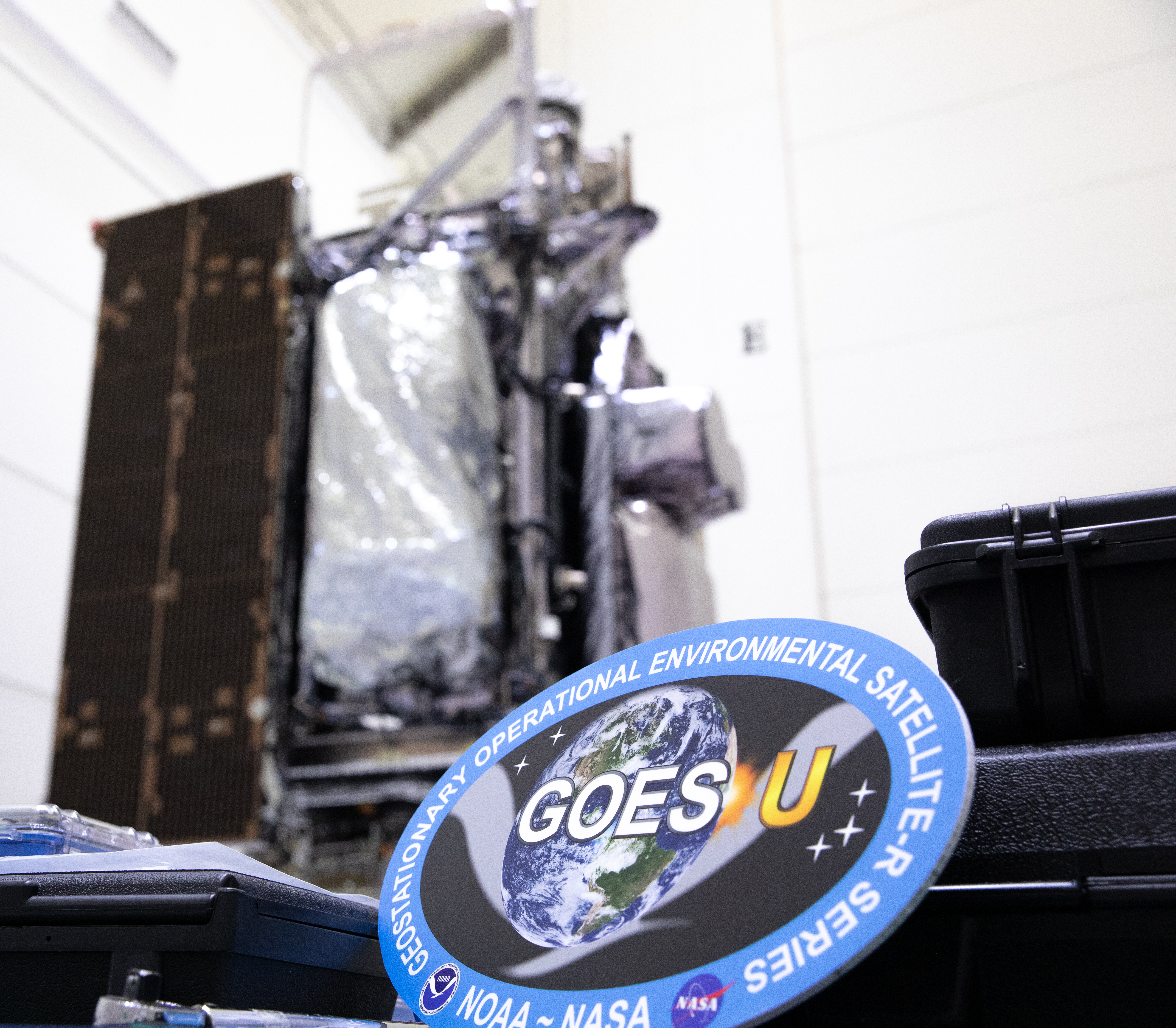
The same attitude-control ideas point Earth-observing satellites such as GOES-19 and Landsat at the planet they measure.
On Saving Planets: GOES-19 · Orbital Mechanics
Sources: NASA Science: NASA to change how it points Hubble Space Telescope (June 4, 2024)
Free learning resources
The lab (Flight dynamics and controls lab)
The lab is the hands-on part of the course. Here it is free and for practice only, with no credit.
Every lab runs in a free simulation or a spreadsheet, so there are no physical hazards. Do not build or fly drones or models for this course. Take screen breaks, sit with good posture, and keep cables out of walkways.
Safety reference: OSHA: Walking-working surfaces (slip, trip and fall hazards)
Lab A: Balancing moments and finding the cg
Week 1
Goal: Balance masses on a plank in PhET Balancing Act, then compute an aircraft-style center of gravity in a spreadsheet.
Procedure
- In PhET Balancing Act, place 10 kg at 1 m on one side and find where 5 kg balances it.
- Record moment = mass × distance on each side.
- In a spreadsheet, list the Unit 1 masses and distances and compute x_cg.
- Add 200 kg at 10 m and recompute.
Data table
| Case | Σm (kg) | x_cg (m) |
|---|---|---|
| Base | 1800 | 4.44 |
| +200 kg at 10 m | 2000 | 5.00 |
Computed sample values.
Sample calculation
- 8000/1800 = 4.44 m.
- 10,000/2000 = 5.00 m.
Safety
- Computer only.
Home or virtual alternative
- Any browser and spreadsheet work.
PhET: Balancing Act · NASA Glenn Beginner’s Guide: Center of gravity
Planet link: NASA Glenn: in flight, airplanes and rockets rotate about their centers of gravity. NASA Glenn Beginner’s Guide: Center of gravity
Lab B: Static margin and trim sweep
Week 3
Goal: Sweep cg position and compute static margin, C_mα and the zero-elevator trim angle.
Procedure
- Use x_np = 0.35c̄, C_Lα = 5.5 /rad, C_m0 = 0.05 (sample values).
- Sweep x_cg from 0.20 to 0.40 c̄.
- Compute SM, C_mα and α_trim.
- Note what happens at and beyond the neutral point.
Data table
| x_cg/c̄ | SM | C_mα (/rad) | α_trim (rad) |
|---|---|---|---|
| 0.20 | 0.15 | −0.825 | 0.0606 |
| 0.25 | 0.10 | −0.55 | 0.0909 |
| 0.30 | 0.05 | −0.275 | 0.182 |
Computed sample values; no stable trim at or aft of the neutral point.
Sample calculation
- C_mα = −5.5 × 0.15 = −0.825.
- α = 0.05/0.275 = 0.182 rad.
Safety
- Computer only.
Home or virtual alternative
- Any spreadsheet works.
NASA Glenn Beginner’s Guide: Aircraft elevator interactive
Planet link: NASA reports the X-59’s stability margin matched predictions in flight. NASA: X-59 aircraft builds momentum through 25th flight (Sept. 4, 2026)
Lab C: Damped oscillation as a second-order mode
Week 6
Goal: Watch damped oscillation in PhET Masses and Springs and compare with the second-order formulas.
Procedure
- In PhET Masses and Springs, hang a mass, add some damping and pull it down.
- Time several cycles and estimate the period and decay.
- In a spreadsheet, compute ω_n, ζ, period and overshoot for m = 0.5 kg, k = 20 N/m, c = 1 N·s/m (sample values).
- Explain how this matches the short-period mode.
Data table
| Quantity | Value |
|---|---|
| ω_n | 6.32 rad/s |
| ζ | 0.158 |
| Damped period | 1.006 s |
| Overshoot | 60.5% |
Computed sample values; simulation readings will differ.
Sample calculation
- ω_n = √40 = 6.32.
- ζ = 1/(2√10) = 0.158.
Safety
- Computer only.
Home or virtual alternative
- Any browser and spreadsheet work.
Planet link: NASA says the X-59 has shown no unexpected instability or excessive vibration. NASA: X-59 aircraft builds momentum through 25th flight (Sept. 4, 2026)
Lab D: Step responses by time-stepping
Week 8
Goal: Simulate first- and second-order step responses with small Euler steps and compare with the formulas.
Procedure
- Simulate ẏ = −2y + 5 from y = 0 with Δt = 0.001 s.
- Simulate ÿ + 2.8ẏ + 16y = 16 from rest.
- Find y(0.5) for the first and the peak and peak time for the second.
- Compare with exact formulas.
Data table
| Quantity | Exact |
|---|---|
| First order y(0.5) | 1.580 |
| Second order peak | 1.309 |
| Peak time | 0.838 s |
| Settling (2%) | 2.86 s |
Computed values; small steps match closely.
Sample calculation
- 2.5(1 − e⁻¹) = 1.580.
- 1 + 0.309 = 1.309.
Safety
- Computer only.
Home or virtual alternative
- Any spreadsheet or Python works.
MIT OpenCourseWare 16.06 Principles of Automatic Control (Fall 2012)
Planet link: NASA’s X-59 team compares flight data with a real-time digital twin. NASA: X-59 aircraft builds momentum through 25th flight (Sept. 4, 2026)
Lab E: Tuning a pitch-attitude autopilot
Week 10
Goal: Compare P and PD control of the plant 1/(s(s + 2)) by simulation.
Procedure
- Simulate θ̈ + 2θ̇ = u with u = K_p(θ_cmd − θ) − K_dθ̇.
- Try K_p = 16, K_d = 0; then K_p = 2.04; then K_p = 16, K_d = 3.6.
- Record overshoot and settling time.
- Choose the best design and explain.
Data table
| Design | Overshoot | Settling (s) |
|---|---|---|
| K_p = 16 | 44.4% | 4.0 |
| K_p = 2.04 | 4.6% | 4.0 |
| K_p = 16, K_d = 3.6 | 4.6% | 1.43 |
Computed from second-order formulas.
Sample calculation
- ζ = 0.25 ⇒ 44.4%; t_s = 4/(0.25 × 4) = 4.0 s.
- PD: t_s = 4/(0.7 × 4) = 1.43 s.
Safety
- Computer only.
Home or virtual alternative
- Any spreadsheet or Python works.
MIT OpenCourseWare 16.30 Feedback Control Systems (Fall 2010)
Planet link: NASA: Dragonfly must fly autonomously at Titan without real-time help from Earth. NASA Science: Dragonfly completes first simulated flight (Oct. 23, 2026)
Lab F: Reaction-wheel slew planner
Week 13
Goal: Plan bang-bang slews for a spacecraft and check peak rates and wheel momentum.
Procedure
- Set I = 1000 kg·m² and τ = 0.5 N·m (sample values).
- Compute slew times for 30°, 90° and 180°.
- Compute the peak rate and the momentum the wheels must absorb.
- Discuss how losing a sensor would change planning.
Data table
| Slew | Time (s) |
|---|---|
| 30° | 64.7 |
| 90° | 112.1 |
| 180° | 158.5 |
Computed sample values.
Sample calculation
- t = 2√(0.5236/0.0005) = 64.7 s.
- t = 2√(3.1416/0.0005) = 158.5 s.
Safety
- Computer only.
Home or virtual alternative
- Any spreadsheet works.
NASA Science: NASA to change how it points Hubble Space Telescope (June 4, 2024)
Planet link: NASA: in one-gyro mode Hubble needs more time to slew and lock onto targets. NASA Science: NASA to change how it points Hubble Space Telescope (June 4, 2024)
Exam prep practice sets
Time yourself: about 10 minutes per problem. Then compare with the full solutions.
Midterm practice set (Units 1–5)
Masses 600 kg at 3 m and 400 kg at 8 m. Find the cg.
Show full solution
- (1800 + 3200)/1000.
Answer: 5.0 m.
x_np = 0.40c̄, x_cg = 0.28c̄, C_Lα = 5 /rad. Find SM and C_mα.
Show full solution
- SM = 0.12.
- −5 × 0.12.
Answer: SM = 0.12; C_mα = −0.60 /rad.
C_m0 = 0.04, C_mα = −0.6, C_mδe = −1.0. Find δ_e to trim at α = 0.05 rad.
Show full solution
- 0.04 − 0.03 − δ_e = 0.
Answer: δ_e = 0.01 rad (0.57°).
Bank angle for a 1500 m radius turn at 80 m/s?
Show full solution
- tan φ = 6400/14,710.
Answer: 23.5°.
Find ω_n and ζ for s² + 3s + 25.
Show full solution
- ω_n = 5; ζ = 3/10.
Answer: ω_n = 5 rad/s; ζ = 0.3.
Final practice set (Units 1–10)
Step response of 4/(s + 4) at t = 0.25 s?
Show full solution
- 1 − e⁻¹.
Answer: 0.632.
Overshoot and settling time for ω_n = 5, ζ = 0.3?
Show full solution
- exp(−0.3π/√0.91).
- 4/1.5.
Answer: 37.2%; 2.67 s.
K on 1/(s(s + 4)) for ζ = 0.5?
Show full solution
- 2ζω_n = 4 ⇒ ω_n = 4.
Answer: K = 16.
Max K for s³ + 3s² + 2s + K?
Show full solution
- 3 × 2 > K.
Answer: K < 6.
Slew time for 60° with α = 0.001 rad/s²?
Show full solution
- 2√(1.0472/0.001).
Answer: 64.7 s.
Momentum of a 0.05 kg·m² wheel at 400 rad/s?
Show full solution
- 0.05 × 400.
Answer: 20 N·m·s.
Formula sheet
Constants
| Constant | Value |
|---|---|
| Standard gravity | g₀ = 9.80665 m/s² |
| 1 radian | 57.2958° |
| 1 ft | 0.3048 m |
| Settling time rule (textbook) | t_s ≈ 4/(ζω_n) for 2% settling |
| First-order step | 63.2% of final value at t = τ |
| Sea-level air density (standard atmosphere) | 1.225 kg/m³ |
Source: NIST Guide to the SI, Appendix B.9: conversion factors
Free texts and simulations
Use these free lectures, NASA guides and simulations alongside the course.
- MIT OpenCourseWare 16.333 Aircraft Stability and Control (Fall 2004): Free MIT stability and control lectures.
- MIT OpenCourseWare 16.06 Principles of Automatic Control (Fall 2012): Free MIT control lectures and problems.
- MIT OpenCourseWare 16.30 Feedback Control Systems (Fall 2010): Free MIT feedback control course.
- NASA Glenn Beginner’s Guide: Aircraft rotations: Free NASA explainer.
- NASA Glenn Beginner’s Guide: Center of gravity: Free NASA explainer.
- PhET: Masses and Springs: Damped oscillation interactively.
Glossary
- Aileron
- Roll control surface.
- Center of gravity
- Average location of mass.
- Damping ratio
- ζ, how fast oscillations decay.
- Dutch roll
- Coupled yaw–roll oscillation.
- Elevator
- Pitch control surface.
- Gain margin
- Gain increase to instability.
- Gyroscope
- Sensor that measures rotation rate.
- Natural frequency
- ω_n of an undamped mode.
- Neutral point
- cg location with neutral pitch stability.
- Overshoot
- Peak above the final value.
- PID controller
- Proportional-integral-derivative control.
- Phase margin
- Extra phase lag to instability.
- Phugoid
- Slow speed–altitude mode.
- Reaction wheel
- Spinning wheel for attitude control.
- Root locus
- Closed-loop pole paths with gain.
- Rudder
- Yaw control surface.
- Short period
- Fast pitch mode.
- Static margin
- Distance from cg to neutral point over chord.
- Transfer function
- Laplace-domain output over input.
- Trim
- Zero net moment.
Self-assessment rubric
No grade or credit is given. Use this to judge honestly where you are in each unit.
| Level | What it looks like |
|---|---|
| 4 · Mastery | Draws axes and block diagrams, picks the right model, checks poles, damping and margins, and explains handling and safety trades in plain words. |
| 3 · Proficient | Solves the practice problems with occasional slips in signs or units. |
| 2 · Developing | Follows worked examples but confuses static and dynamic stability or ω_n and ω_d. |
| 1 · Beginning | Plugs numbers into formulas without a diagram; needs to revisit the unit. |
Suggested weighting if you want a score
| Part | Weight |
|---|---|
| Practice problems | 20% |
| Labs | 25% |
| Midterm practice set | 25% |
| Final practice set | 30% |
Aim for level 3 or better in every unit before moving to the next course.