

Calculus I
Limits, derivatives, optimization, integrals and the Fundamental Theorem, with four computer labs on real-world rates of change. Free, self-paced, and tied to real planet-saving work.
Courses › MATH 110
About this course
This is a free self-study course outline written by Saving Planets. It is not a university course, it carries no academic credit, and no school is involved.
Its scope follows first-semester college calculus (single-variable differential calculus and an introduction to integrals), modeled on the topics and depth of open materials such as OpenStax Calculus Volume 1 and MIT OpenCourseWare 18.01SC Single Variable Calculus, which we link to throughout. Those organizations do not endorse this page.
What we add: every unit connects calculus to real climate, energy and spaceflight problems, every number on the page is re-computed by a checking script before it goes live, and four computer labs let you do calculus on data the way scientists and engineers do.
Work through it in order. Each unit has goals, key ideas, equations, step-by-step examples, practice with full answers, common mistakes, flashcards and a quiz. Your progress is saved only in this browser.
How this course helps save the planet
Calculus is the mathematics of change. Climate scientists use derivatives to turn a record of carbon dioxide or sea ice into a rate of change, engineers use optimization to get the most energy from wind and the most mission from every kilogram of rocket fuel, and integrals add up power into energy.
Each unit ends with a short, sourced section showing how its ideas help both people and nature.
Before you start
Prerequisites
- Algebra: factoring, rational expressions, solving equations and inequalities.
- Functions and graphs: domain, range, composition, inverse functions.
- Trigonometry: radians, the unit circle, sine, cosine, tangent and basic identities.
- Exponential and logarithmic functions, including e and ln.
How to study
- Read the unit, then close it and try the worked examples yourself before checking each step.
- Do every practice problem on paper before opening the answer.
- Sketch a graph whenever you can. Most calculus mistakes show up as a picture that makes no sense.
- Check derivatives by estimating the slope numerically, and integrals by estimating the area.
- Use a graphing tool such as Desmos to test your intuition, never to replace the work.
- Retake the quizzes a few days later. Spaced practice beats one long session.
Lab equipment (for the wet labs)
- A computer or tablet with a spreadsheet (Google Sheets, Excel or LibreOffice).
- A free graphing calculator such as Desmos.
- Optional: Python with NumPy, for those who want to code the labs.
Suggested 15-week schedule
About 6 to 9 hours a week: reading, practice problems and, in lab weeks, the lab.
| Week | Unit | Topics | Reading |
|---|---|---|---|
| 1 | Functions & Limits | Functions review; the idea of a limit; limits from graphs and tables | OpenStax 1.1–1.5, 2.1–2.2 |
| 2 | Functions & Limits | Limit laws; algebraic techniques; special trigonometric limits | OpenStax 2.3 |
| 3 | Functions & Limits | Limits at infinity; asymptotes; the precise definition | OpenStax 2.5, 4.6 |
| 4 | Continuity & the Derivative | Continuity, the IVT, the derivative; Lab A | OpenStax 2.4, 3.1–3.2 |
| 5 | Differentiation Rules | Power, product and quotient rules; higher derivatives | OpenStax 3.3–3.4 |
| 6 | Differentiation Rules | Trigonometric derivatives; the chain rule | OpenStax 3.5–3.6 |
| 7 | Differentiation Rules | Implicit differentiation; exponential and log derivatives; midterm practice | OpenStax 3.7–3.9 |
| 8 | Applications I: Related Rates, Approximation & Newton’s Method | Related rates; linear approximation and differentials | OpenStax 4.1–4.2 |
| 9 | Applications I: Related Rates, Approximation & Newton’s Method | L’Hôpital’s rule; Newton’s method; Lab B | OpenStax 4.8–4.9 |
| 10 | Applications II: Extrema, Graph Shape & Optimization | Extrema, the Mean Value Theorem, graph shape | OpenStax 4.3–4.5 |
| 11 | Applications II: Extrema, Graph Shape & Optimization | Applied optimization; Lab C | OpenStax 4.7 |
| 12 | Integrals & the Fundamental Theorem of Calculus | Riemann sums and the definite integral | OpenStax 5.1–5.2 |
| 13 | Integrals & the Fundamental Theorem of Calculus | The Fundamental Theorem; Lab D | OpenStax 5.3–5.4 |
| 14 | Integrals & the Fundamental Theorem of Calculus | Substitution; average value; areas between curves | OpenStax 5.5, 6.1 |
| 15 | Review | Review and final practice set | All units |
Your progress
Tick units and labs as you finish them, and take the quizzes. Progress and quiz scores are saved only in this browser, never sent to us.
Turn on JavaScript to track progress.
Unit 1 · Weeks 1–3
Functions & Limits
A limit describes what a function approaches. It is the idea underneath every derivative and integral.
Learning objectives
By the end of this unit you can:
- Estimate limits from graphs and tables, including one-sided limits.
- Evaluate limits with the limit laws, factoring and rationalizing.
- Find limits at infinity and identify horizontal and vertical asymptotes.
- State the precise (ε–δ) definition of a limit.
Key concepts
- lim f(x) as x → a = L means f(x) can be made as close to L as we like by taking x close enough to a, but not equal to a.
- A limit exists only if the left- and right-hand limits agree.
- For a 0/0 form, simplify first: factor, cancel, or multiply by a conjugate.
- Two special limits: sin x / x → 1 and (1 − cos x)/x → 0 as x → 0 (x in radians).
- At infinity, compare the highest powers in a rational function.
Key equations
Worked examples, step by step
Example 1.1 Find lim (x² − 4)/(x − 2) as x → 2.
Show the steps
- Direct substitution gives 0/0, so simplify.
- (x² − 4)/(x − 2) = (x − 2)(x + 2)/(x − 2) = x + 2 for x ≠ 2.
- Now substitute: 2 + 2 = 4.
Answer: 4.
Example 1.2 Find lim (√(x + 4) − 2)/x as x → 0.
Show the steps
- 0/0 again. Multiply top and bottom by the conjugate √(x + 4) + 2.
- Top becomes (x + 4) − 4 = x, so the expression is 1/(√(x + 4) + 2).
- Substitute x = 0: 1/(2 + 2) = 1/4.
Answer: 1/4.
Example 1.3 Find lim (3x² + 1)/(2x² − 5) as x → ∞.
Show the steps
- Divide top and bottom by x²: (3 + 1/x²)/(2 − 5/x²).
- As x → ∞, 1/x² → 0.
Answer: 3/2, so y = 3/2 is a horizontal asymptote.
Practice problems
Work each on paper first, then check.
lim (x² − 9)/(x − 3) as x → 3
Show answer
Factor: x + 3 → 6.
lim (5x + 2)/(x − 1) as x → ∞
Show answer
Divide by x: 5.
lim (1 − cos x)/x as x → 0
Show answer
0 (a standard limit).
lim 1/x as x → 0⁺ and as x → 0⁻
Show answer
+∞ from the right, −∞ from the left, so the two-sided limit does not exist.
lim sin(3x)/x as x → 0
Show answer
Write it as 3 · sin(3x)/(3x) → 3 × 1 = 3.
Common misconceptions
Myth: A limit is just the value of the function at that point.
Actually: The limit ignores f(a). f can be undefined at a and still have a limit there, as in Example 1.1.
Myth: 0/0 means the limit is 0 (or does not exist).
Actually: 0/0 is an indeterminate form: the limit could be anything. You have to simplify.
Myth: If the graph gets close to a line, it can never cross it.
Actually: A graph can cross a horizontal asymptote; the asymptote describes behavior far away.
Flashcards
Limit
The value f(x) approaches as x approaches a.
One-sided limit
Limit from the left (x → a⁻) or right (x → a⁺).
Indeterminate form
0/0 or ∞/∞: simplify before deciding.
Horizontal asymptote
y = L when f(x) → L as x → ±∞.
Vertical asymptote
x = a when f(x) → ±∞ as x → a.
ε–δ definition
For every ε > 0 there is δ > 0 that keeps f(x) within ε of L.
Self-check quiz
How this helps save the planet
Every climate record is a list of measurements at separate times. The idea of a limit, shrinking the time step toward zero, is what lets scientists talk about the rate of change at an instant rather than just over a year or a decade.
NOAA has measured carbon dioxide at Mauna Loa Observatory since 1958. Its data pages publish both the concentration and its yearly growth rate, a direct use of the average rate of change that limits make precise.
On Saving Planets: OCO-2: measuring CO₂ from orbit
Sources: NOAA GML: trends in atmospheric CO₂ · NOAA GML: CO₂ growth rates
Free learning resources
- OpenStax Calculus 1, 2.2 The Limit of a Function: Free textbook section.
- OpenStax Calculus 1, 2.3 The Limit Laws: Limit laws with worked examples.
- OpenStax Calculus 1, 2.5 The Precise Definition of a Limit: ε–δ proofs.
- MIT OpenCourseWare 18.01SC Single Variable Calculus: Free MIT lectures, notes and problem sets.
Unit 2 · Week 4
Continuity & the Derivative
Continuity means no breaks. The derivative is the limit of average rates of change: the slope of the tangent line.
Learning objectives
By the end of this unit you can:
- Test a function for continuity and use the Intermediate Value Theorem.
- Compute a derivative from the limit definition.
- Interpret a derivative as a slope, a velocity and a rate of change, with units.
- Write the equation of a tangent line.
Key concepts
- f is continuous at a if f(a) is defined, the limit exists, and they are equal.
- Intermediate Value Theorem: a continuous function on [a, b] takes every value between f(a) and f(b).
- The derivative f′(a) is the limit of the difference quotient [f(a + h) − f(a)]/h as h → 0.
- Units of f′ are units of f per unit of x: meters per second, ppm per year.
- A function is not differentiable at a corner, a cusp, a vertical tangent or a break.
Key equations
Worked examples, step by step
Example 2.1 Use the definition to find the derivative of f(x) = x².
Show the steps
- [(x + h)² − x²]/h = (2xh + h²)/h = 2x + h.
- As h → 0 this tends to 2x.
Answer: f′(x) = 2x.
Example 2.2 Find the tangent line to y = x³ at x = 1.
Show the steps
- y′ = 3x², so the slope at x = 1 is 3.
- Point: (1, 1).
- y − 1 = 3(x − 1), so y = 3x − 2.
Answer: y = 3x − 2.
Example 2.3 For what a is f(x) = x + 1 (x < 1), ax² (x ≥ 1) continuous everywhere?
Show the steps
- Left limit at 1: 1 + 1 = 2.
- Right value and limit: a × 1² = a.
- Continuity needs a = 2.
Answer: a = 2.
Practice problems
Work each on paper first, then check.
Use the definition to differentiate f(x) = 1/x.
Show answer
[1/(x + h) − 1/x]/h = −1/(x(x + h)) → −1/x².
A dropped stone falls s(t) = 4.9t² meters. Find its average velocity from t = 1 to t = 3 s and its instantaneous velocity at t = 2 s.
Show answer
Average: (44.1 − 4.9)/2 = 19.6 m/s. Instantaneous: s′(t) = 9.8t, so 19.6 m/s at t = 2.
Show that x³ + x − 1 = 0 has a root between 0 and 1.
Show answer
f(0) = −1 < 0 and f(1) = 1 > 0, and f is continuous, so by the IVT it crosses 0 in between.
Is f(x) = |x| differentiable at 0?
Show answer
No. The slope is −1 from the left and +1 from the right, so the limit of the difference quotient does not exist (a corner).
Common misconceptions
Myth: Continuous means differentiable.
Actually: |x| is continuous at 0 but has no derivative there. Differentiable does imply continuous, though.
Myth: The derivative is the change in y.
Actually: It is the rate of change: change in y per unit change in x, in the limit.
Myth: The tangent line touches the curve at only one point.
Actually: It can cross the curve elsewhere, and even at the point of tangency (as for y = x³ at 0).
Flashcards
Continuity at a
lim f(x) as x → a equals f(a).
Intermediate Value Theorem
Continuous on [a, b] ⇒ every value between f(a) and f(b) is taken.
Difference quotient
[f(x + h) − f(x)]/h, an average rate of change.
Derivative
Limit of the difference quotient; instantaneous rate of change.
Tangent line
y = f(a) + f′(a)(x − a).
Differentiable ⇒ continuous
But not the other way round.
Self-check quiz
How this helps save the planet
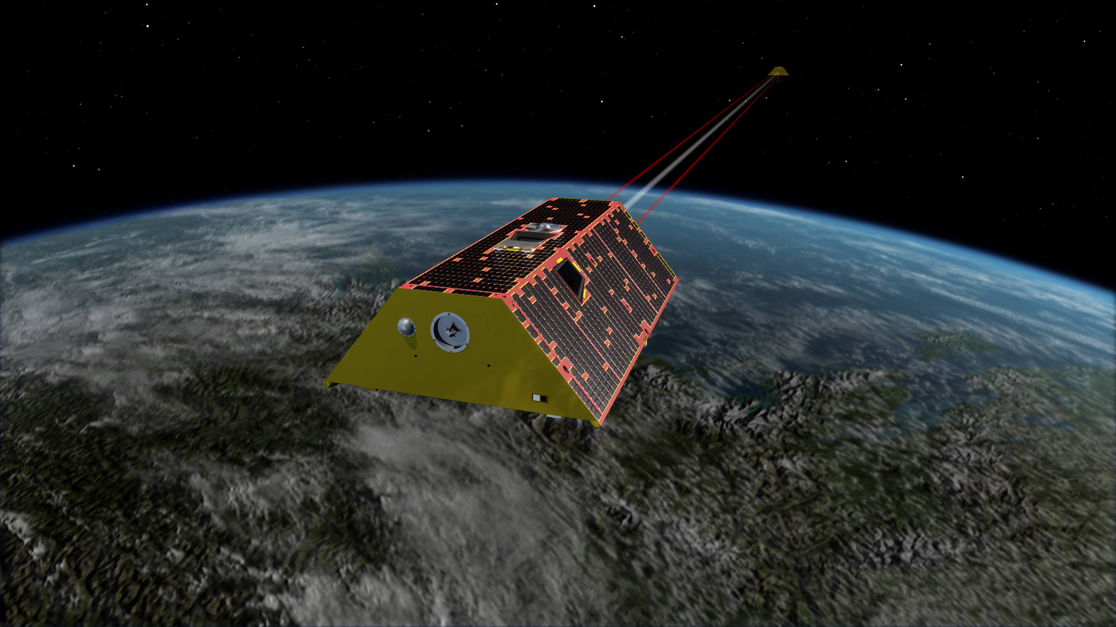
The derivative turns a position record into a speed. Satellite navigation does this constantly: GRACE-FO, for example, measures how the distance between its two satellites changes, and those changes reveal shifts in water and ice on Earth.
Rates with units are how climate change is reported in practice: parts per million of CO₂ per year, millimeters of sea level per year. Reading a derivative with its units is a core science-literacy skill.
On Saving Planets: GRACE-FO · Physics I + Lab
Sources: NASA JPL: GRACE-FO · OpenStax Calculus 1, 3.1 Defining the Derivative
Free learning resources
- OpenStax Calculus 1, 2.4 Continuity: Continuity and the IVT.
- OpenStax Calculus 1, 3.1 Defining the Derivative: The derivative from first principles.
- PhET: Calculus Grapher: See a function and its derivative together.
Unit 3 · Weeks 5–7
Differentiation Rules
Power, product, quotient and chain rules, plus derivatives of trigonometric, exponential and logarithmic functions, and implicit differentiation.
Learning objectives
By the end of this unit you can:
- Differentiate polynomials, products, quotients and compositions quickly and correctly.
- Differentiate sin, cos, tan, eˣ and ln x.
- Use implicit differentiation to find dy/dx.
- Find higher derivatives and interpret the second derivative as acceleration.
Key concepts
- Power rule: d/dx xⁿ = nxⁿ⁻¹ for any real n.
- Product rule: (fg)′ = f′g + fg′. Quotient rule: (f/g)′ = (f′g − fg′)/g².
- Chain rule: the derivative of f(g(x)) is f′(g(x)) · g′(x), outside derivative times inside derivative.
- eˣ is its own derivative; ln x has derivative 1/x. That is why e appears in every growth and decay model.
- Implicit differentiation: differentiate both sides with respect to x, treating y as a function of x.
Key equations
Worked examples, step by step
Example 3.1 Differentiate y = x² sin x.
Show the steps
- Product rule with f = x², g = sin x.
- y′ = 2x sin x + x² cos x.
Answer: y′ = 2x sin x + x² cos x.
Example 3.2 Differentiate y = (3x² + 1)⁵.
Show the steps
- Outside: u⁵ → 5u⁴. Inside: u = 3x² + 1 → 6x.
- y′ = 5(3x² + 1)⁴ · 6x.
Answer: y′ = 30x(3x² + 1)⁴.
Example 3.3 Find the slope of the circle x² + y² = 25 at (3, 4).
Show the steps
- Differentiate: 2x + 2y y′ = 0.
- y′ = −x/y = −3/4.
Answer: −3/4.
Practice problems
Work each on paper first, then check.
d/dx (3x⁴ − 5x² + 7)
Show answer
12x³ − 10x.
d/dx ln(x² + 1)
Show answer
2x/(x² + 1) (chain rule).
d/dx (x/(x + 1))
Show answer
[(x + 1) − x]/(x + 1)² = 1/(x + 1)².
A quantity grows as Q(t) = 1000e^(0.02t). How fast is it growing at t = 0, and what is its relative growth rate?
Show answer
Q′(t) = 20e^(0.02t), so 20 units per unit time at t = 0. Q′/Q = 0.02, a constant 2% per unit time.
If s(t) = t³ − 6t², find the velocity and acceleration at t = 1.
Show answer
v = 3t² − 12t = −9; a = 6t − 12 = −6.
Common misconceptions
Myth: The derivative of a product is the product of the derivatives.
Actually: Use the product rule: (fg)′ = f′g + fg′.
Myth: d/dx sin(3x) = cos(3x).
Actually: Chain rule: 3 cos(3x).
Myth: d/dx eˣ = x eˣ⁻¹.
Actually: The power rule does not apply to variable exponents. d/dx eˣ = eˣ.
Flashcards
Power rule
d/dx xⁿ = nxⁿ⁻¹.
Product rule
(fg)′ = f′g + fg′.
Quotient rule
(f/g)′ = (f′g − fg′)/g².
Chain rule
[f(g(x))]′ = f′(g(x)) g′(x).
d/dx eˣ
eˣ.
d/dx ln x
1/x.
Self-check quiz
How this helps save the planet
Growth and decay models built on eˣ describe population growth, radioactive decay used to date ice cores, and compound growth in emissions. The chain rule gives their rates of change in one step.
A relative growth rate (Q′/Q) is how scientists compare changes in quantities of very different sizes, for example how fast a forest area or a greenhouse gas is changing as a percentage per year.
On Saving Planets: Deforestation hub · Earth observation
Sources: OpenStax Calculus 1, 3.9 Derivatives of Exponential and Logarithmic Functions · NASA: carbon dioxide vital sign
Free learning resources
- OpenStax Calculus 1, 3.3 Differentiation Rules: Power, product and quotient rules.
- OpenStax Calculus 1, 3.5 Derivatives of Trigonometric Functions: Trigonometric derivatives.
- OpenStax Calculus 1, 3.6 The Chain Rule: Chain rule with many examples.
- OpenStax Calculus 1, 3.8 Implicit Differentiation: Implicit differentiation.
Unit 4 · Weeks 8–9
Applications I: Related Rates, Approximation & Newton’s Method
Use derivatives to link changing quantities, approximate hard values, evaluate tricky limits and solve equations numerically.
Learning objectives
By the end of this unit you can:
- Solve related-rates problems.
- Use linear approximation and differentials to estimate values and errors.
- Apply L’Hôpital’s rule to 0/0 and ∞/∞ forms.
- Solve equations with Newton’s method.
Key concepts
- Related rates: write an equation linking the quantities, differentiate with respect to time, then substitute values.
- Near x = a, f(x) ≈ f(a) + f′(a)(x − a): the tangent line is the best straight-line estimate.
- L’Hôpital’s rule: for 0/0 or ∞/∞, lim f/g = lim f′/g′ if the right side exists.
- Newton’s method: xₙ₊₁ = xₙ − f(xₙ)/f′(xₙ). It usually converges very fast from a good starting guess.
Key equations
Worked examples, step by step
Example 4.1 A spherical weather balloon’s radius grows at 2 cm/s. How fast is its volume growing when r = 10 cm?
Show the steps
- V = (4/3)πr³, so dV/dt = 4πr² dr/dt.
- dV/dt = 4π × 10² × 2 = 800π ≈ 2,513 cm³/s.
Answer: About 2,510 cm³/s.
Example 4.2 Estimate √4.1 with a linear approximation.
Show the steps
- f(x) = √x, a = 4: f(4) = 2, f′(4) = 1/(2√4) = 1/4.
- L(4.1) = 2 + (1/4)(0.1) = 2.025.
Answer: 2.025 (the true value is 2.02485…).
Example 4.3 Use Newton’s method to solve x² = 2 starting from x₀ = 1.
Show the steps
- f(x) = x² − 2, f′(x) = 2x, so xₙ₊₁ = xₙ − (xₙ² − 2)/(2xₙ).
- x₁ = 1.5, x₂ = 1.416667, x₃ = 1.414216.
Answer: x₃ = 1.414216, already correct to 6 significant figures (√2 = 1.4142136…).
Practice problems
Work each on paper first, then check.
A 5 m ladder slides down a wall; its foot moves away at 0.5 m/s. How fast is the top falling when the foot is 3 m from the wall?
Show answer
x² + y² = 25, so x x′ + y y′ = 0. With x = 3, y = 4: y′ = −(3/4)(0.5) = −0.375 m/s, falling at 0.375 m/s.
lim (eˣ − 1)/x as x → 0
Show answer
L’Hôpital: eˣ/1 → 1.
Newton’s method for x³ − 2x − 5 = 0 from x₀ = 2. Find x₁ and x₂.
Show answer
f(2) = −1, f′(2) = 10, so x₁ = 2.1. f(2.1) = 0.061, f′(2.1) = 11.23, so x₂ = 2.0946.
Use differentials to estimate the change in the area of a 10 cm radius disk if the radius grows by 0.1 cm.
Show answer
dA = 2πr dr = 2π × 10 × 0.1 = 2π ≈ 6.28 cm².
Common misconceptions
Myth: L’Hôpital means differentiating the quotient f/g.
Actually: Differentiate the top and bottom separately, and only for 0/0 or ∞/∞ forms.
Myth: In related rates, plug in the numbers first, then differentiate.
Actually: Differentiate first; substituting too early turns variables into constants with zero derivative.
Myth: Newton’s method always finds a root.
Actually: A bad starting point, or f′ near zero, can send it off or make it cycle.
Flashcards
Related rates
Differentiate an equation linking quantities with respect to t.
Linear approximation
f(x) ≈ f(a) + f′(a)(x − a).
Differential
dy = f′(x) dx.
L’Hôpital’s rule
For 0/0 or ∞/∞: lim f/g = lim f′/g′.
Newton’s method
xₙ₊₁ = xₙ − f(xₙ)/f′(xₙ).
Quadratic convergence
Newton’s method roughly doubles the correct digits each step near a simple root.
Self-check quiz
How this helps save the planet
Predicting where a satellite will be means solving Kepler’s equation, M = E − e sin E, for E. It has no algebraic solution, so it is commonly solved numerically, often with Newton’s method, as in Lab B. Accurate orbit prediction keeps Earth-observing satellites safely apart and their images correctly placed on the map.
Weather balloons, like the one in Example 4.1, carry instruments that measure the atmosphere for weather forecasts; related rates link how fast they rise and expand.
On Saving Planets: Orbits guide · Orbital period calculator
Sources: OpenStax Calculus 1, 4.9 Newton’s Method · OpenStax University Physics 1, 13.5 Kepler’s Laws
Free learning resources
- OpenStax Calculus 1, 4.1 Related Rates: Free textbook section.
- OpenStax Calculus 1, 4.2 Linear Approximations and Differentials: Tangent-line estimates and error.
- OpenStax Calculus 1, 4.8 L’Hôpital’s Rule: Indeterminate forms.
- OpenStax Calculus 1, 4.9 Newton’s Method: Iterative root finding.
Unit 5 · Weeks 10–11
Applications II: Extrema, Graph Shape & Optimization
Find maxima and minima, read a graph’s shape from f′ and f″, and solve real design problems by optimization.
Learning objectives
By the end of this unit you can:
- Find critical points and absolute extrema on a closed interval.
- State and use the Mean Value Theorem.
- Use the first and second derivative tests and find inflection points.
- Set up and solve applied optimization problems.
Key concepts
- Critical points are where f′ = 0 or f′ does not exist. Extrema of a smooth function happen there or at endpoints.
- Mean Value Theorem: on a smooth interval, the instantaneous rate equals the average rate somewhere.
- f′ > 0 means increasing; f″ > 0 means concave up. An inflection point is where concavity changes.
- Optimization recipe: draw it, write the quantity to optimize as a function of one variable using the constraint, differentiate, find critical points, check endpoints.
Key equations
Worked examples, step by step
Example 5.1 Find the local extrema of f(x) = x³ − 3x.
Show the steps
- f′(x) = 3x² − 3 = 0 at x = ±1.
- f″(x) = 6x: f″(−1) = −6 < 0 (max), f″(1) = 6 > 0 (min).
- f(−1) = 2, f(1) = −2.
Answer: Local max 2 at x = −1; local min −2 at x = 1.
Example 5.2 A closed cylindrical can must hold 500 cm³. What radius uses the least metal?
Show the steps
- Constraint: πr²h = 500, so h = 500/(πr²).
- Area A = 2πr² + 2πrh = 2πr² + 1000/r.
- A′ = 4πr − 1000/r² = 0 gives r³ = 500/(2π), r = 4.30 cm.
- Then h = 8.60 cm = 2r, and A = 349 cm².
Answer: r = 4.30 cm, h = 8.60 cm (height equals diameter).
Example 5.3 In the simplest model of a wind turbine, the fraction of wind power captured is Cp = 4a(1 − a)², where a is how much the rotor slows the wind. Find the maximum.
Show the steps
- Cp′ = 4(1 − a)² − 8a(1 − a) = 4(1 − a)(1 − 3a).
- Critical points a = 1 and a = 1/3; a = 1 gives Cp = 0.
- Cp(1/3) = 4 × (1/3) × (2/3)² = 16/27 = 0.593.
Answer: 59.3%: the Betz limit, the theoretical maximum for any wind turbine.
Practice problems
Work each on paper first, then check.
A farmer has 100 m of fence for three sides of a rectangle along a river. What is the largest area?
Show answer
A = x(100 − 2x); A′ = 100 − 4x = 0 at x = 25. Area = 25 × 50 = 1,250 m².
Find the absolute max and min of f(x) = x² − 4x on [0, 5].
Show answer
Critical point x = 2: f = −4. Endpoints: f(0) = 0, f(5) = 5. Max 5, min −4.
Verify the MVT for f(x) = x² on [1, 3].
Show answer
Average rate (9 − 1)/2 = 4; f′(c) = 2c = 4 at c = 2, inside [1, 3].
Where is f(x) = x³ − 6x² concave up?
Show answer
f″ = 6x − 12 > 0 when x > 2; inflection point at x = 2.
Common misconceptions
Myth: f′(c) = 0 always means a max or min.
Actually: x³ has f′(0) = 0 but no extremum there.
Myth: The absolute max is always at a critical point.
Actually: On a closed interval it can be at an endpoint. Always check them.
Myth: Concave up means increasing.
Actually: Concavity is about f″; a function can be concave up and decreasing, like e⁻ˣ.
Flashcards
Critical point
f′ = 0 or undefined.
Extreme Value Theorem
Continuous on [a, b] ⇒ absolute max and min exist.
Mean Value Theorem
f′(c) = [f(b) − f(a)]/(b − a) for some c.
First derivative test
Sign change of f′ from + to − is a max; − to + is a min.
Concavity
f″ > 0 up, f″ < 0 down.
Betz limit
Max Cp = 16/27 ≈ 59.3%.
Self-check quiz
How this helps save the planet
Optimization is engineering. The Betz limit in Example 5.3 comes from one derivative set to zero, and it tells wind engineers the most any turbine could ever extract from the wind.
Mission designers optimize too: a Hohmann transfer is usually the most fuel-efficient two-burn route between two circular orbits, and less propellant means smaller, cheaper launches for climate and weather satellites.
Using the least material for a job, like the can in Example 5.2, cuts the energy and resources that go into making it.
On Saving Planets: Hohmann transfer calculator · Physics I, Unit 4: wind power
Sources: U.S. DOE: How do wind turbines work? · OpenStax Calculus 1, 4.7 Applied Optimization Problems
Free learning resources
- OpenStax Calculus 1, 4.3 Maxima and Minima: Extrema and critical points.
- OpenStax Calculus 1, 4.5 Derivatives and the Shape of a Graph: First and second derivative tests.
- OpenStax Calculus 1, 4.7 Applied Optimization Problems: Many solved design problems.
Unit 6 · Weeks 12–14
Integrals & the Fundamental Theorem of Calculus
Integrals add up tiny pieces: area, distance, energy. The Fundamental Theorem links them to derivatives.
Learning objectives
By the end of this unit you can:
- Approximate areas with Riemann sums and the trapezoid rule.
- Define the definite integral and use its properties.
- Use both parts of the Fundamental Theorem of Calculus.
- Find antiderivatives, including by substitution, and compute net change, average value and areas between curves.
Key concepts
- A Riemann sum adds f(xᵢ)Δx over small slices; the definite integral is its limit as the slices shrink.
- FTC part 1: d/dx ∫ₐˣ f(t) dt = f(x). Integration and differentiation undo each other.
- FTC part 2: ∫ₐᵇ f(x) dx = F(b) − F(a) for any antiderivative F.
- Net change theorem: integrating a rate gives the total change. Integrating power gives energy; integrating velocity gives displacement.
- Substitution is the chain rule in reverse.
Key equations
Worked examples, step by step
Example 6.1 Find ∫₀² x² dx.
Show the steps
- Antiderivative x³/3.
- 8/3 − 0 = 8/3.
Answer: 8/3 ≈ 2.667.
Example 6.2 Find ∫₀¹ 2x(x² + 1)³ dx.
Show the steps
- Let u = x² + 1, du = 2x dx; u goes from 1 to 2.
- ∫₁² u³ du = [u⁴/4]₁² = (16 − 1)/4.
Answer: 15/4 = 3.75.
Example 6.3 A solar array’s output on a clear day is modeled as P(t) = 5 sin(πt/12) kW for 0 ≤ t ≤ 12 hours after sunrise. How much energy does it make?
Show the steps
- Energy = ∫₀¹² 5 sin(πt/12) dt.
- Antiderivative: −(60/π) cos(πt/12).
- −(60/π)(cos π − cos 0) = 120/π.
Answer: 120/π ≈ 38.2 kWh (a simplified model, not a real array).
Practice problems
Work each on paper first, then check.
∫₀^π sin x dx
Show answer
[−cos x]₀^π = 1 + 1 = 2.
d/dx ∫₀ˣ cos(t²) dt
Show answer
cos(x²), by FTC part 1.
A rocket’s upward velocity is v(t) = 9.8t m/s for 3 s. How far does it rise?
Show answer
∫₀³ 9.8t dt = 4.9 × 9 = 44.1 m.
Find the area between y = x and y = x² on [0, 1].
Show answer
∫₀¹ (x − x²) dx = 1/2 − 1/3 = 1/6.
Find the average value of f(x) = x² on [0, 3].
Show answer
(1/3) ∫₀³ x² dx = (1/3)(9) = 3.
Common misconceptions
Myth: An integral is always an area, so it is always positive.
Actually: It is a signed area: parts below the axis count as negative. ∫₀^{2π} sin x dx = 0.
Myth: Forgetting + C does not matter.
Actually: For indefinite integrals the constant is part of the answer; it matters whenever an initial condition is given.
Myth: In substitution, keep the old limits.
Actually: Change the limits to u-values, or substitute back before evaluating.
Flashcards
Riemann sum
Σ f(xᵢ*) Δx; an area estimate.
Definite integral
Limit of Riemann sums; signed area.
FTC part 1
d/dx ∫ₐˣ f = f(x).
FTC part 2
∫ₐᵇ f = F(b) − F(a).
Net change
Integral of a rate = total change.
Substitution
u = g(x), du = g′(x) dx: the chain rule in reverse.
Self-check quiz
How this helps save the planet
Energy is the integral of power over time. Grid planners add up hour-by-hour solar and wind output this way to know how much clean energy they will get and how much storage they need.
Satellite instruments measure rates, such as the flow of sunlight or of water, and integrals turn those rates into totals: how much energy Earth absorbs, or how much water a river basin gains or loses over a season.
The numerical integration in Lab D is exactly how real data, which comes as separate measurements, gets integrated.
On Saving Planets: GRACE-FO · Calculators
Sources: OpenStax Calculus 1, 5.3 The Fundamental Theorem of Calculus · U.S. DOE: How do wind turbines work?
Free learning resources
- OpenStax Calculus 1, 5.1 Approximating Areas: Riemann sums.
- OpenStax Calculus 1, 5.2 The Definite Integral: Definition and properties.
- OpenStax Calculus 1, 5.3 The Fundamental Theorem of Calculus: Both parts with proofs.
- OpenStax Calculus 1, 5.5 Substitution: u-substitution.
- OpenStax Calculus 1, 6.1 Areas between Curves: Areas between curves.
Computer labs
Calculus has no wet lab, so this course has four short computer labs instead. Each one applies a unit to real-world style data with a spreadsheet: finite differences, Newton’s method, optimization and numerical integration.
These are the same numerical methods engineers and climate scientists use every day. The sample data in each lab is for practice; each lab links to the real data source.
Safety reference: NOAA Global Monitoring Laboratory: trends in CO₂
Lab A: Rates of change from data
Week 4
Goal: Estimate a rate of change and its acceleration from a table of measurements, the way climate scientists treat a CO₂ record.
Procedure
- Enter the sample table in a spreadsheet.
- Compute forward differences (rate over each year) and central differences.
- Compute the second difference: is the rate itself rising?
- Download real annual means from NOAA and repeat; compare with NOAA’s published growth rates.
Data table
| Year t | C (ppm) |
|---|---|
| 0 | 400.0 |
| 1 | 402.4 |
| 2 | 404.9 |
| 3 | 407.5 |
| 4 | 410.2 |
Sample values for practice, not real measurements. Use NOAA’s data for the real thing.
Sample calculation
- Central difference at t = 2: (407.5 − 402.4)/2 = 2.55 ppm per year.
- Second difference at t = 2: 407.5 − 2(404.9) + 402.4 = 0.1 ppm per year².
- A positive second difference means the growth rate is itself increasing (in this sample).
Safety
- Keep a copy of the raw data untouched; do calculations in new columns.
Home or virtual alternative
- Everything here is done on a computer or even by hand.
Planet link: Rates of change are how CO₂ trends are reported and compared. NOAA GML: trends in atmospheric CO₂
Lab B: Newton’s method and Kepler’s equation
Week 9
Goal: Solve Kepler’s equation M = E − e sin E for a satellite’s eccentric anomaly E, the key step in predicting where it is.
Procedure
- Set M = 1.0 rad and e = 0.1 in a spreadsheet; start with E₀ = M.
- Fill down the Newton formula for four rows.
- Watch how many digits stop changing each step.
- Try e = 0.9 and E₀ = M: how many steps does it need now?
Data table
| Step n | Eₙ (rad) |
|---|---|
| 0 | 1.000000 |
| 1 | 1.088953 |
| 2 | 1.088598 |
| 3 | 1.088598 |
Computed values (M = 1.0 rad, e = 0.1).
Sample calculation
- f(E) = E − 0.1 sin E − 1; f′(E) = 1 − 0.1 cos E.
- From E₀ = 1: E₁ = 1.088953, E₂ = 1.088598, after which the first 7 digits stop changing.
- Check: 1.088598 − 0.1 sin(1.088598) = 1.000000.
Safety
- None beyond normal computer use.
Home or virtual alternative
- A spreadsheet or Desmos is enough.
OpenStax Calculus 1, 4.9 Newton’s Method
Planet link: Orbit prediction keeps Earth-observing satellites safe and their data correctly placed.
Lab C: Optimizing a wind turbine
Week 11
Goal: Confirm the Betz limit numerically and by calculus.
Procedure
- Tabulate Cp for a = 0 to 0.5 in steps of 0.05 and graph it.
- Find the highest value in the table.
- Solve Cp′(a) = 0 by hand and compare.
Data table
| a | Cp |
|---|---|
| 0.20 | 0.512 |
| 0.30 | 0.588 |
| 1/3 | 0.593 |
| 0.40 | 0.576 |
Computed values from the model.
Sample calculation
- Cp(0.3) = 4 × 0.3 × 0.7² = 0.588.
- Cp(1/3) = 16/27 = 0.593, the maximum.
- Real turbines capture less because of drag, wake rotation and tip losses.
Safety
- None beyond normal computer use.
Home or virtual alternative
- A spreadsheet or Desmos is enough.
U.S. DOE: How do wind turbines work?
Planet link: Knowing the ceiling tells engineers how much improvement is still possible.
Lab D: Numerical integration of solar power
Week 13
Goal: Integrate a power curve with the midpoint and trapezoid rules and compare with the exact answer.
Procedure
- Model P(t) = 5 sin(πt/12) kW on 0 ≤ t ≤ 12 h.
- With n = 6 slices (Δt = 2 h), compute the midpoint and trapezoid sums.
- Compare with the exact 120/π kWh. Double n and watch the errors shrink.
Data table
| Method (n = 6) | Energy (kWh) |
|---|---|
| Midpoint | 38.64 |
| Trapezoid | 37.32 |
| Exact (FTC) | 38.20 |
Model values, not data from a real array.
Sample calculation
- Trapezoid: 2 × [0 + 2(2.5 + 4.330 + 5 + 4.330 + 2.5)]/2 = 37.32 kWh.
- Midpoint: 2 × Σ P at t = 1, 3, …, 11 = 38.64 kWh.
- Errors: midpoint +0.44, trapezoid −0.88. The midpoint error is about half the trapezoid error, with opposite sign, as theory predicts.
Safety
- None beyond normal computer use.
Home or virtual alternative
- A spreadsheet or Desmos is enough.
OpenStax Calculus 1, 5.1 Approximating Areas
Planet link: This is how real, hourly energy data is added up to plan clean power and storage.
Exam prep practice sets
Time yourself: about 10 minutes per problem. Then compare with the full solutions.
Midterm practice set (Units 1–3)
Find lim (x − 4)/(√x − 2) as x → 4.
Show full solution
- Multiply by √x + 2: (x − 4)(√x + 2)/(x − 4) = √x + 2.
- Substitute x = 4: 2 + 2.
Answer: 4.
Differentiate y = x³eˣ and evaluate at x = 1.
Show full solution
- Product rule: y′ = 3x²eˣ + x³eˣ = (3x² + x³)eˣ.
- At x = 1: 4e.
Answer: 4e ≈ 10.87.
Find the tangent line to y = ln x at x = 1.
Show full solution
- y(1) = 0, y′ = 1/x = 1.
- y − 0 = 1(x − 1).
Answer: y = x − 1.
Differentiate y = sin(3x²).
Show full solution
- Chain rule: cos(3x²) · 6x.
Answer: y′ = 6x cos(3x²).
Final practice set (all units)
Water flows into a cylindrical tank of radius 2 m at 0.5 m³/min. How fast does the level rise?
Show full solution
- V = πr²h = 4πh, so dV/dt = 4π dh/dt.
- dh/dt = 0.5/(4π).
Answer: About 0.0398 m/min (4.0 cm per minute).
Find ∫₁ᵉ (1/x) dx.
Show full solution
- [ln x]₁ᵉ = 1 − 0.
Answer: 1.
Find ∫₀⁴ √x dx.
Show full solution
- Antiderivative (2/3)x^(3/2).
- (2/3)(8) = 16/3.
Answer: 16/3 ≈ 5.33.
A rectangle has perimeter 40 m. What dimensions maximize its area?
Show full solution
- A = x(20 − x); A′ = 20 − 2x = 0 at x = 10.
Answer: A 10 m × 10 m square, area 100 m².
Use L’Hôpital to find lim x²/eˣ as x → ∞.
Show full solution
- ∞/∞: → 2x/eˣ, still ∞/∞.
- → 2/eˣ → 0.
Answer: 0: exponentials outgrow any power.
Formula sheet
Constants
| Constant | Value |
|---|---|
| e | 2.718281828… |
| π | 3.141592654… |
| ln 2 | 0.693147… |
| 1 radian | 57.2958° |
Graphing and data tools
Use these free tools and data sources alongside the course.
- Desmos graphing calculator: Graph functions, sliders and tangent lines in the browser.
- PhET: Calculus Grapher: Draw a function and see its derivative and integral.
- NOAA: trends in atmospheric CO₂: Real Mauna Loa and global CO₂ data to practice rates of change.
Glossary
- Antiderivative
- A function F with F′ = f.
- Asymptote
- A line a graph approaches far out or near a blow-up.
- Chain rule
- Derivative of a composition: outside′ × inside′.
- Concavity
- Direction a graph bends; sign of f″.
- Continuity
- No breaks: the limit equals the function value.
- Critical point
- Where f′ is zero or undefined.
- Definite integral
- Signed area under a curve between two limits.
- Derivative
- Instantaneous rate of change; slope of the tangent line.
- Differential
- dy = f′(x) dx.
- Fundamental Theorem of Calculus
- Links derivatives and integrals; ∫ₐᵇ f = F(b) − F(a).
- Indeterminate form
- 0/0 or ∞/∞; needs more work.
- Inflection point
- Where concavity changes.
- Limit
- The value a function approaches.
- Linear approximation
- Tangent-line estimate.
- Mean Value Theorem
- Instantaneous rate equals average rate somewhere.
- Newton’s method
- Iterative root finder using tangent lines.
- Optimization
- Finding the best value of a quantity under constraints.
- Riemann sum
- Sum of rectangle areas approximating an integral.
- Substitution
- Integration technique reversing the chain rule.
- Trapezoid rule
- Numerical integration with trapezoids.
Self-assessment rubric
No grade or credit is given. Use this to judge honestly where you are in each unit.
| Level | What it looks like |
|---|---|
| 4 · Mastery | Solves unseen problems, justifies each step with a rule or theorem, and checks answers with a graph or estimate. |
| 3 · Proficient | Solves the practice problems correctly with occasional algebra slips. |
| 2 · Developing | Follows worked examples but struggles to choose a method, or misapplies the chain rule. |
| 1 · Beginning | Memorizes formulas without knowing when they apply; needs to revisit the unit. |
Suggested weighting if you want a score
| Part | Weight |
|---|---|
| Practice problems | 30% |
| Computer labs | 15% |
| Midterm practice set | 25% |
| Final practice set | 30% |
Aim for level 3 or better in every unit before moving to the next course.